Six functions are available for fitting linear models or linear mixed effects models. These can be used instead of simple ANOVAs or ‘mixed’ ANOVAs when there are random factors to consider.
These functions rely on lm and lmer (latter implemented in package lmerTest).
This page examples of using linear mixed-effects models to get the:
- ANOVA table (
mixed_anova,mixed_anova_slopes) with F and P values - Fitted model (
mixed_model,mixed_model_slopes), which is useful for diagnostics and posthoc comparisons.
Both fit the full model with interaction terms when more than one fixed factors are provided. By default, variable intercepts only models are fit. For simplicity, grafify currently implements one version of variable slopes model through mixed_model_slopes and mixed_anova_slopes. Refer to lme4 package for more complex analyses with random effects.
Type II sum of squaress
ANOVA tables show type II sum of squares (type II SS). ANOVA tables with mixed_anova are generated using the anova() call through lmerTest that adds P values.
If you want Type III SS, first set contrasts using options(contrasts=c("contr.sum", "contr.poly") before fitting the model or getting the ANOVA table. Fitting the model without this and setting type = "III" will give incorrect results. The default contrasts in R can be obtained by running options(contrasts=c("contr.treatment", "contr.poly")).
Data format
See the data help page and ensure data table is in the long-format, and check that you have correctly converted categorical variables with as.factor and columns with numeric variables are in the correct format.
Examples used here
We will use data_1w_death and data_2w_Festing in these examples. In this vignette we use ordinary linear models; see the vignette on mixed-effects models for analyses of the same data where the random factor is taken into account.
Let’s look at these data first so you have an idea of whether or not there are differences between them.
First the data_1w_death (one-way ANOVA design) data from 5 independent in vitro experiments where death of host cells was measured (as percentage of total cells) after infection with three different strains of a pathogenic bacterium (factor Genotype).
head(data_1w_death, n = 6) #see first 6 rows of data#> Experiment Genotype Death
#> 1 Exp_1 WT 25.012173
#> 2 Exp_1 KO_1 1.824973
#> 3 Exp_1 KO_2 14.294956
#> 4 Exp_2 WT 16.542609
#> 5 Exp_2 KO_1 2.131199
#> 6 Exp_2 KO_2 23.749439A plot of these data shows that KO_1 induces very little death as compared to the other two bacterial strains.
plot_3d_scatterbox(data_1w_death, #data
                   Genotype,      #fixed factor
                   Death,         #Y variable
                   Experiment)    #shapes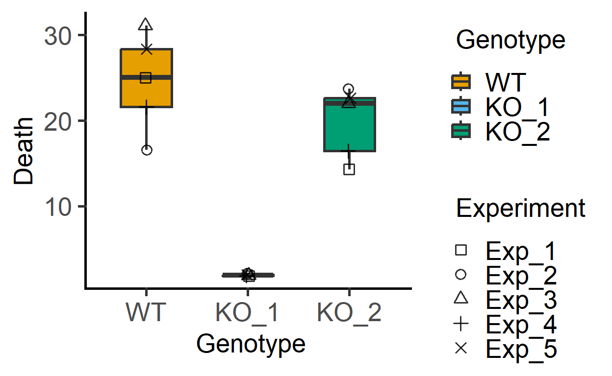
The data_2w_Festing data from Festing et al dataset has two fixed factors (“Treatment” & “Strain”). For the present analysis, I will ignore the blocking factor (“Block”), and we use the same data set in the vignette on mixed effects models (mixed_anova).
head(data_2w_Festing, n = 8) #see first 8 rows#> Block Treatment Strain GST
#> 1 A Control NIH 444
#> 2 A Treated NIH 614
#> 3 A Control BALB/C 423
#> 4 A Treated BALB/C 625
#> 5 A Control A/J 408
#> 6 A Treated A/J 856
#> 7 A Control 129/Ola 447
#> 8 A Treated 129/Ola 719The plot below of these data suggests that Treatment generally increases GST values irrespective of the mouse Strain (although the magnitude of increase appears to be different across the strains).
plot_4d_scatterbox(data_2w_Festing, #data
                   Strain,          #factor 1
                   GST,             #Y  variable
                   Treatment,       #factor 2
                   Block)           #shapes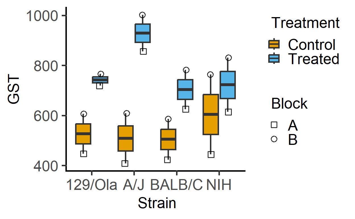
Let’s fit a linear model, use diagnostics and get ANOVA table.
In this vignette we use linear mixed-effects models; see the vignette on ordinary linear models for analyses of the same data where the random factor is ignored.
mixed_model
mixed_model to save models for diagnostics and posthoc_ functions. The mixed_model and mixed_anova calls have identically arguments.
Mixed effects one-way ANOVA
mod_1wdeath <- mixed_model(data_1w_death,      #data table
                           "Death",            #quantitative variable
                           "Genotype",         #fixed factor
                           "Experiment")              #random factor

#diagnostic residual plot
plot_qqmodel(mod_1wdeath)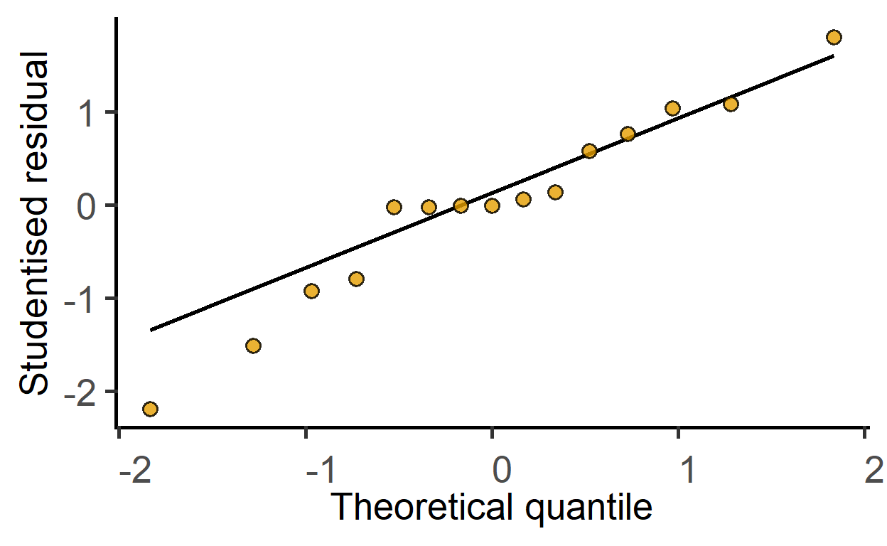
Mixed effects two-way ANOVA
mod_2w <- mixed_model(data_2w_Festing,
                      "GST",
                      c("Strain", "Treatment"),
                      "Block")

mod_2wtdeath <- mixed_model(data_2w_Tdeath,
                            "logit(PI/100)",     #logit transformation in formula
                            c("Genotype", "Time"),
                            c("Experiment", "Subject"))
Check model residuals with the plot_qqmodel function.
plot_qqmodel(mod_2w) #saved above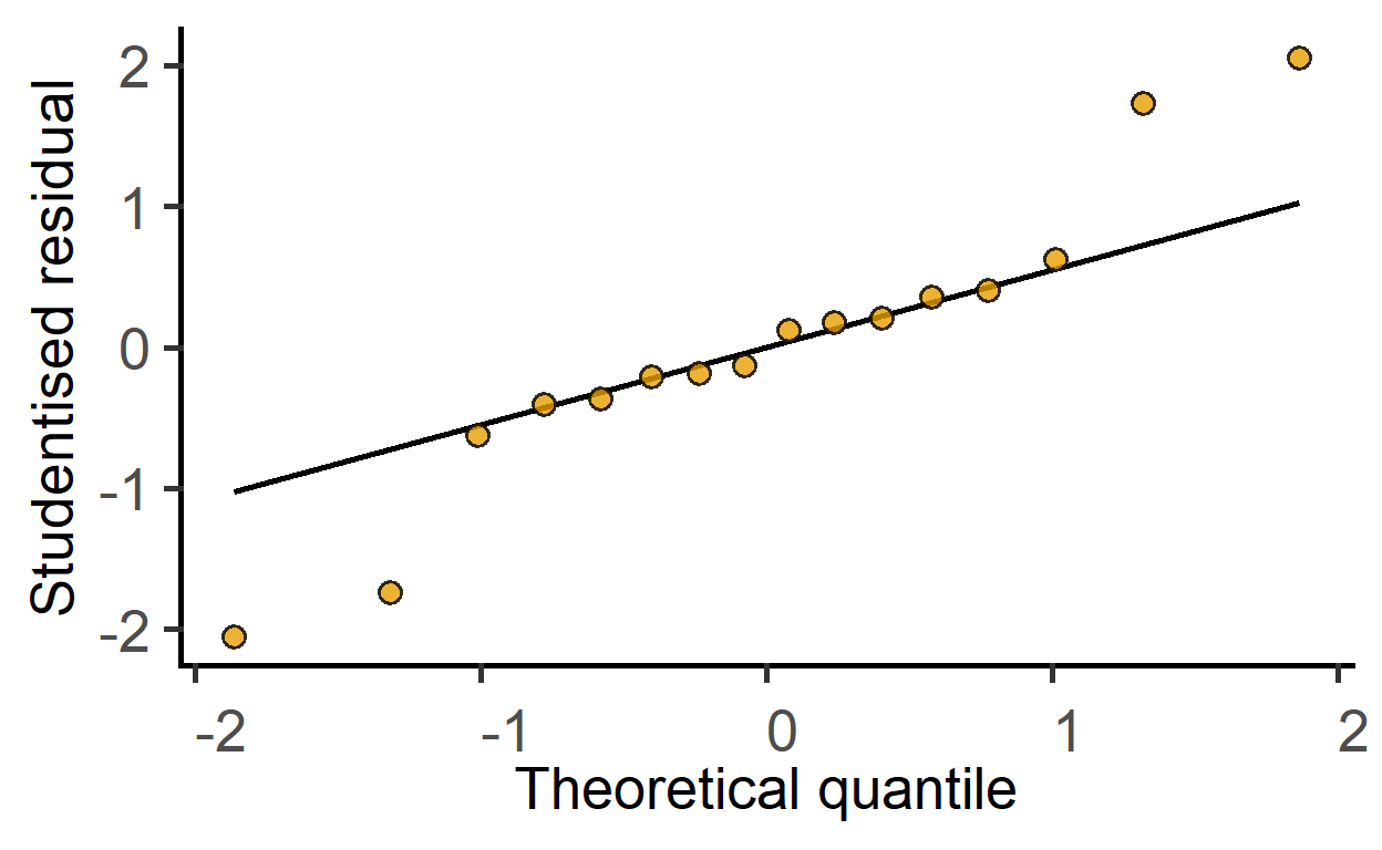
plot_qqmodel(mod_2wtdeath)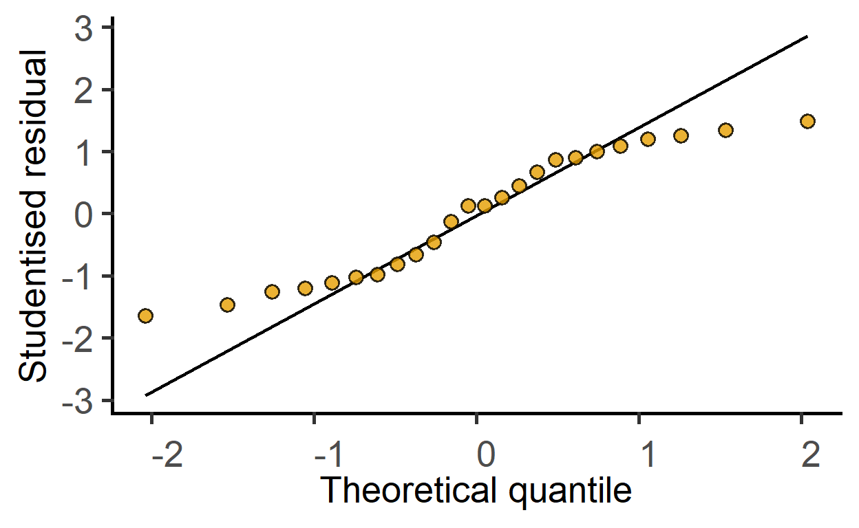
The ggResidPanel package is great for model diagnostics. Check it out.
mixed_anova
One-way ANOVA & randomised blocks
ANOVA table with random factor taken into account.
mixed_anova(data_1w_death,      #data table
            "Death",            #quantitative variable
            "Genotype",         #fixed factor
            "Experiment")       #random factor
#> Type II Analysis of Variance Table with Kenward-Roger's method
#> Sum Sq Mean Sq NumDF DenDF F value Pr(>F)
#> Genotype 1420.2 710.1 2 8 42.659 5.401e-05 ***
#> ---
#> Signif. codes: 0 '***' 0.001 '**' 0.01 '*' 0.05 '.' 0.1 ' ' 1The output indicates a huge impact of Genotype on cell death. Compare this result with the ordinary linear model.
Two-way ANOVA & randomised blocks
Let’s analyse the Festing et al dataset this time including the random factor (analysis as ordinary linear model here).
mixed_anova(data_2w_Festing,            #data table
            "GST",                      #quantitative variable
            c("Strain", "Treatment"),   #fixed factors
            "Block")                    #random factor
#> Type II Analysis of Variance Table with Kenward-Roger's method
#> Sum Sq Mean Sq NumDF DenDF F value Pr(>F)
#> Strain 28613 9538 3 7 3.2252 0.09144 .
#> Treatment 227529 227529 1 7 76.9394 5.041e-05 ***
#> Strain:Treatment 49591 16530 3 7 5.5897 0.02832 *
#> ---
#> Signif. codes: 0 '***' 0.001 '**' 0.01 '*' 0.05 '.' 0.1 ' ' 1The effect of Treatment looks more marked, and there may be a hint of interaction, so dig deeper!
Currently, grafify implements one type of variable slopes model (mixed_model_slopes and mixed_anova_slopes). Refer to lme4 package to fit other kinds of random effects.
Two-way ANOVA, repeated-measures & randomised blocks
The two-way repeated-measures data_2w_Tdeath has two fixed factors (Genotype & Time) and two random factors, Experiment and Subject. The Subject indicates repeated-measure over Time. The data table also has a column with numeric “Time2” column that could be used for graphs, remember to use the column with categorical “Time” column for analysis.
#>   Experiment Time Subject Genotype       PI Time2
#> 1         e1 t100      s1       WT 20.47120   100
#> 2         e2 t100      s2       WT 28.88967   100
#> 3         e3 t100      s3       WT 11.55061   100
#> 4         e4 t100      s4       WT 23.24516   100
#> 5 e5 t100 s5 WT 30.20904 100str(data_2w_Tdeath) #Time coded as categorical variable#> 'data.frame': 24 obs. of 6 variables:
#> $ Experiment: Factor w/ 6 levels "e1","e2","e3",..: 1 2 3 4 5 6 1 2 3 4 ...
#> $ Time : Factor w/ 2 levels "t100","t300": 1 1 1 1 1 1 1 1 1 1 ...
#> $ Subject : Factor w/ 12 levels "s1","s10","s11",..: 1 5 6 7 8 9 10 11 12 2 ...
#> $ Genotype : Factor w/ 2 levels "WT","KO": 1 1 1 1 1 1 2 2 2 2 ...
#> $ PI : num 20.5 28.9 11.6 23.2 30.2 ...
#> $ Time2 : int 100 100 100 100 100 100 100 100 100 100 ...mixed_anova(data_2w_Tdeath, #data table
"logit(PI/100)", #logit transformation in formula
c("Genotype", "Time"), #fixed factors
c("Experiment", "Subject")) #random factors#> Type II Analysis of Variance Table with Kenward-Roger's method
#> Sum Sq Mean Sq NumDF DenDF F value Pr(>F)
#> Genotype 1.18171 1.18171 1 5 58.5419 0.0006071 ***
#> Time 1.84830 1.84830 1 10 91.5646 2.377e-06 ***
#> Genotype:Time 0.08288 0.08288 1 10 4.1059 0.0702377 .
#> ---
#> Signif. codes: 0 '***' 0.001 '**' 0.01 '*' 0.05 '.' 0.1 ' ' 1Results show a large effect of Genotype & Time, and questionable interaction effect.
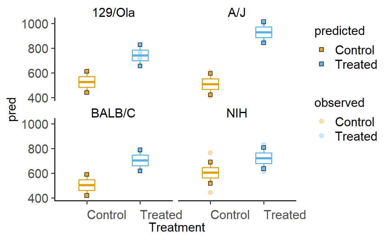
Plotting model-predicted data
The function plot_lm_predict is handy to check how close the values predicted from the linear model are to observed (or measured) values that were used to fit the model. A good model will predict numbers close to observed/real data.
This function takes in a fitted model, and needs X and Y variables that exactly match those used to fit the model.
Let us plot the predictions of models fitted above.
#plots for Festing data set
plot_lm_predict(Model = mod_2w,  #fitted model
                xcol = Treatment,  #one independent factor
                ycol = GST, #dependent variable
                ByFactor = Strain) #second factor