Colours in grafify
All plot_ functions have arguments that apply different grafify palette and colour options directly. Vignettes of plot_ functions describe how to do this.
This vignette describes scale_fill_grafify and scale_colour_grafify which can be used with any ggplot2 graph.
This vignette explains the scale_fill_ and scale_colour_ functions in grafify to apply grafify colour schemes on any ggplot2 object.
Since v2.3.0, grafify offers twelve colour blind-friendly palettes are available for nominal or categorical or discreet variables, with 4-20 colours per scheme.
Five schemes are available for quantitative data, including three sequential or continuous and two divergent schemes.
These are based on schemes by Paul Tol, Okabe-Ito, Mike Mol’s blog, and cols4all package).

scale_fill_ and scale_colour_ (or scale_color_)
These functions from grafify can be used to add colours to any ggplot2 object. The default fill/colour scale will add the okabe_ito palette. This only works when the variable is discrete/nominal, and throw up an error if the variable is numeric. Use one of the quantitative palettes when there’s an error.
Discrete/nominal/categorical colour schemes available:
okabe_ito, bright, contrast, dark, kelly, light, muted, pale, r4, safe, vibrant
Sequential colour schemes
grey_conti, blue_conti, yellow_conti
Divergent quantitative palettes
OrBl_div, PrGn_div
There are only 3 arguments, palette, ColSeq (logical) and reverse (logical).
Use ColSeq = FALSE to get the most distant colours in the palette rather sequential colours from the chosen palette (default is TRUE).
Applying scale_colour_grafify:
This example uses the InsectSprays dataset in R (try str(InsectSprays) to see it has 6 levels of one factor “spray” and “count” as the response variable).
ggplot(data = InsectSprays,         #data table
        aes(x = spray, y = count))+
  geom_point(size = 3,
             aes(colour = spray))+
  scale_colour_grafify()+  #default settings
  labs(title = "scale_colour_grafify",
       subtitle = "(default `okabe_ito` palette)")+
  theme_classic(base_size = 21)
Reversing colour order:
ggplot(data = InsectSprays,         #data table
        aes(x = spray, y = count))+
  geom_point(size = 3,
             aes(colour = spray))+
  scale_colour_grafify(reverse = TRUE)+ #reversed colour, default palette
  labs(title = "scale_colour_grafify",
       subtitle = "reverse `okabe_ito` palette")+
  theme_classic(base_size = 21)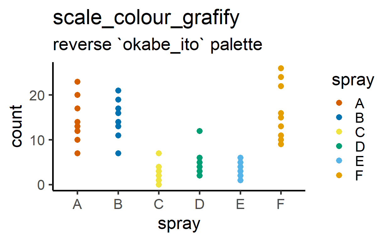
Picking distant colours
Set the ColSeq argument to FALSE to not pick sequential colours.
ggplot(data = InsectSprays,         #data table
        aes(x = spray, y = count))+
  geom_point(size = 3,
             aes(colour = spray))+
  scale_colour_grafify(ColSeq = FALSE)+ #not sequential colours
  labs(title = "scale_colour_grafify",
       subtitle = "`ColSeq = FALSE`")+
  theme_classic(base_size = 21)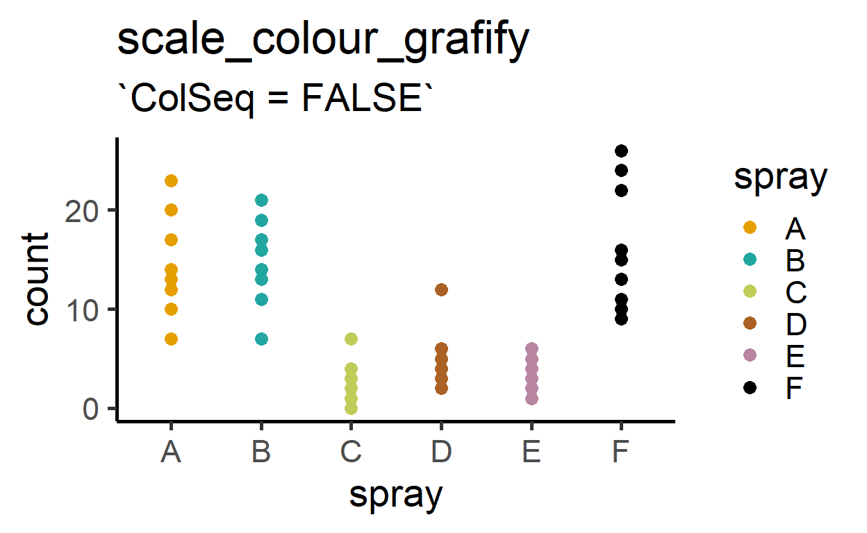
Quantitative palettes
(in v2.3 and earlier, this needed the discrete argument, but this has been dropped. ).
There are five palettes available:
Sequential quantitative palettes:
grey_conti, blue_conti, yellow_conti
Divergent quantitative palettes:
OrBl_div, PrGn_div
Here are examples on a quantitative variable using the mtcars data set in R.
ggplot(mtcars, aes(x = mpg, y = disp))+
  geom_point(aes(fill = gear),
             size = 4, shape = 21)+
  scale_fill_grafify(palette = "blue_conti")+ #blue_conti scheme
  theme_classic(base_size = 21)+
  labs("`blue_conti` colour scheme")+
  theme_classic(base_size = 21)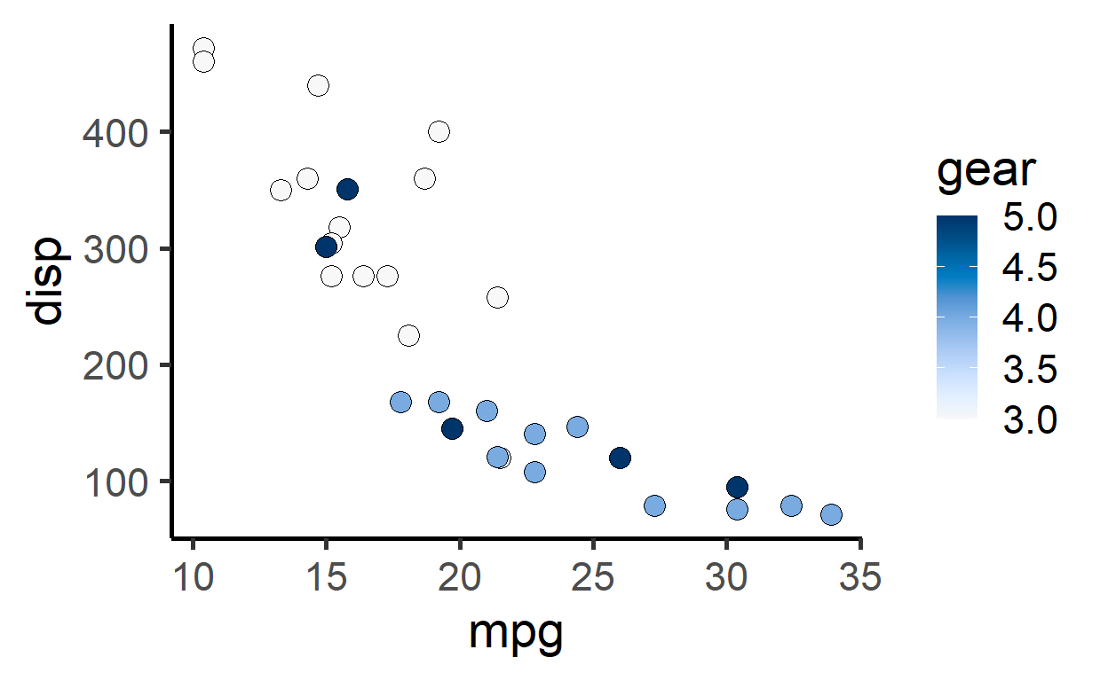
ggplot(mtcars, aes(x = mpg, y = disp))+
  geom_point(aes(fill = gear),
             size = 4, shape = 21)+
  scale_fill_grafify(palette = "yellow_conti")+ #yellow_conti scheme
  theme_classic(base_size = 21)+
  labs("`yellow_conti` colour scheme")+
  theme_classic(base_size = 21)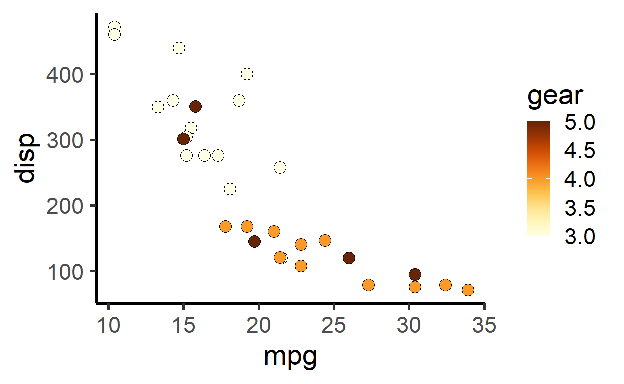
Viewing grafify palettes and hexcodes
Palettes can be quickly viewed, along with hexcodes, using the plot_grafify_palette call.
plot_grafify_palette(palette = "okabe_ito") 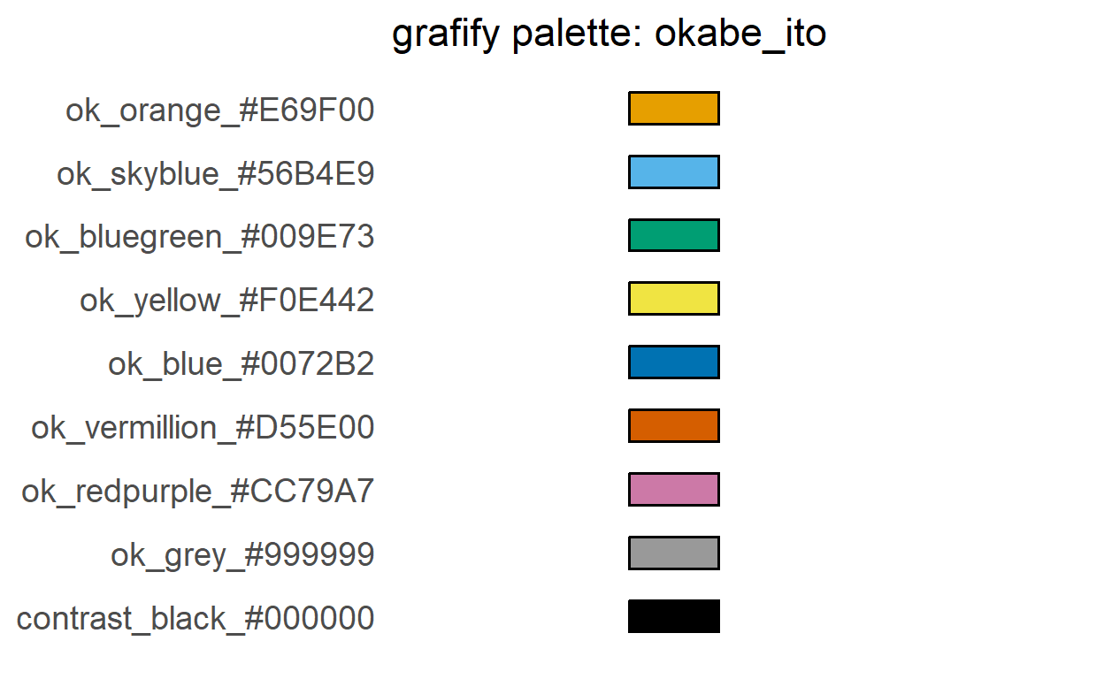
plot_grafify_palette(palette = "kelly")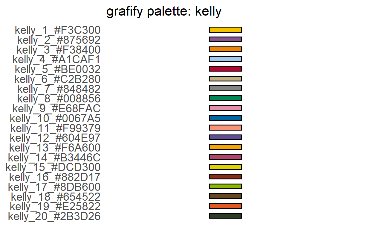
You can get the value of the hexcodes if you want to manually apply these colours to other objects in R, for example with scale_colour_manual.
Here is the list of hex codes of all the colours in the palettes.
grafify:::graf_palettes#> $okabe_ito
#> ok_orange ok_skyblue ok_bluegreen ok_yellow
#> "#E69F00" "#56B4E9" "#009E73" "#F0E442"
#> ok_blue ok_vermillion ok_redpurple ok_grey
#> "#0072B2" "#D55E00" "#CC79A7" "#999999"
#> contrast_black
#> "#000000"
#>
#> $bright
#> bright_red bright_blue bright_yellow bright_green bright_cyan
#> "#ee6677" "#4477aa" "#ccbb44" "#228833" "#66ccee"
#> bright_purple bright_grey
#> "#aa3377" "#bbbbbb"
#>
#> $contrast
#> contrast_black contrast_white contrast_yellow contrast_red
#> "#000000" "#ffffff" "#ddaa33" "#bb5566"
#> contrast_blue
#> "#004488"
#>
#> $dark
#> dark_blue dark_cyan dark_yellow dark_green dark_red
#> "#222255" "#225555" "#666633" "#225522" "#663333"
#> dark_grey
#> "#555555"
#>
#> $fishy
#> fishy_1 fishy_2 fishy_3 fishy_4 fishy_5 fishy_6 fishy_7
#> "#6388b4" "#ffae34" "#ef6f6a" "#8cc2ca" "#c3bc3f" "#55ad89" "#bb7693"
#> fishy_8 fishy_9
#> "#baa094" "#767676"
#>
#> $kelly
#> kelly_1 kelly_2 kelly_3 kelly_4 kelly_5 kelly_6 kelly_7
#> "#F3C300" "#875692" "#F38400" "#A1CAF1" "#BE0032" "#C2B280" "#848482"
#> kelly_8 kelly_9 kelly_10 kelly_11 kelly_12 kelly_13 kelly_14
#> "#008856" "#E68FAC" "#0067A5" "#F99379" "#604E97" "#F6A600" "#B3446C"
#> kelly_15 kelly_16 kelly_17 kelly_18 kelly_19 kelly_20
#> "#DCD300" "#882D17" "#8DB600" "#654522" "#E25822" "#2B3D26"
#>
#> $light
#> light_orange light_blue light_yellow light_pink light_cyan
#> "#ee8866" "#77aadd" "#eedd88" "#ffaabb" "#99ddff"
#> light_mint light_pear light_olive pale_grey
#> "#44bb99" "#bbcc33" "#aaaa00" "#dddddd"
#>
#> $muted
#> muted_rose muted_indigo muted_sand muted_green muted_cyan
#> "#cc6677" "#332288" "#ddcc77" "#117733" "#88ccee"
#> muted_wine muted_teal muted_olive muted_purple pale_grey
#> "#882255" "#44aa99" "#999933" "#aa4499" "#dddddd"
#>
#> $pale
#> pale_blue pale_cyan pale_green pale_yellow pale_red
#> "#bbccee" "#cceeff" "#ccddaa" "#eeeebb" "#ffcccc"
#> pale_grey
#> "#dddddd"
#>
#> $r4
#> r4_1 r4_2 r4_3 r4_4 r4_5 r4_6
#> "#DF536B" "#61D04F" "#2297E6" "#28E2E5" "#CD0BBC" "#F5C710"
#>
#> $safe
#> safe_blue safe_red safe_yellow safe_green
#> "#88CCEE" "#CC6677" "#DDCC77" "#117733"
#> safe_violet safe_purple safe_bluegreen safe_bush
#> "#332288" "#AA4499" "#44AA99" "#999933"
#> safe_reddish safe_wine safe_skyblue
#> "#882255" "#661100" "#6699CC"
#>
#> $vibrant
#> vibrant_orange vibrant_blue vibrant_magenta vibrant_cyan
#> "#ee7733" "#0077bb" "#ee3377" "#33bbee"
#> vibrant_red vibrant_teal bright_grey
#> "#cc3311" "#009988" "#bbbbbb"
#>
#> $OrBl_div
#> OrBl_1 OrBl_2 OrBl_3 OrBl_4 OrBl_5 OrBl_6 OrBl_7
#> "#9E3D21" "#BE4E21" "#DA6524" "#EF8530" "#F0AC72" "#D8D4C9" "#A2BCCF"
#> OrBl_8 OrBl_9 OrBl_10 OrBl_11
#> "#6FA3CB" "#5789B6" "#4071A0" "#2B5B8A"
#>
#> $PrGn_div
#> PrGn_1 PrGn_2 PrGn_3 PrGn_4 PrGn_5 PrGn_6 PrGn_7
#> "#762A83" "#9262A2" "#B18FC0" "#D0B7D8" "#EADAEB" "#F7F7F7" "#DFF1DA"
#> PrGn_8 PrGn_9 PrGn_10 PrGn_11
#> "#BEDEB2" "#8CC485" "#4EA258" "#1A7837"
#>
#> $blue_conti
#> blue_1 blue_2 blue_3 blue_4 blue_5 blue_6 blue_7
#> "#F8F8F8" "#E5F1FF" "#D0E4FF" "#B6D2F8" "#99BFEE" "#79ABE1" "#5294D3"
#> blue_8 blue_9 blue_10 blue_11
#> "#027EC4" "#0066A5" "#004C85" "#00356C"
#>
#> $grey_conti
#> grey_lin1 grey_lin2 grey_lin3 grey_lin4 grey_lin5 grey_lin6
#> "#F1F1F1" "#D8D8D8" "#C0C0C0" "#A9A9A9" "#929292" "#7D7D7D"
#> grey_lin7 grey_lin8 grey_lin9 grey_lin10 grey_lin11
#> "#676767" "#535353" "#3F3F3F" "#2C2C2C" "#1A1A1A"
#>
#> $yellow_conti
#> YlOrBr_1 YlOrBr_2 YlOrBr_3 YlOrBr_4 YlOrBr_5 YlOrBr_6 YlOrBr_7
#> "#FFFFE5" "#FFF7BC" "#FEE391" "#FEC44F" "#FB9A29" "#EC7014" "#CC4C02"
#> YlOrBr_8 YlOrBr_9
#> "#993404" "#662506"
#>
#> $all_grafify
#> ok_orange ok_skyblue ok_bluegreen ok_yellow
#> "#E69F00" "#56B4E9" "#009E73" "#F0E442"
#> ok_blue ok_vermillion ok_redpurple muted_indigo
#> "#0072B2" "#D55E00" "#CC79A7" "#332288"
#> muted_cyan muted_teal muted_green muted_olive
#> "#88ccee" "#44aa99" "#117733" "#999933"
#> muted_sand muted_rose muted_wine muted_purple
#> "#ddcc77" "#cc6677" "#882255" "#aa4499"
#> light_blue light_cyan light_mint light_pear
#> "#77aadd" "#99ddff" "#44bb99" "#bbcc33"
#> light_olive light_yellow light_orange light_pink
#> "#aaaa00" "#eedd88" "#ee8866" "#ffaabb"
#> pale_blue pale_cyan pale_green pale_yellow
#> "#bbccee" "#cceeff" "#ccddaa" "#eeeebb"
#> pale_red pale_grey dark_grey bright_grey
#> "#ffcccc" "#dddddd" "#555555" "#bbbbbb"
#> ok_grey contrast_white contrast_yellow contrast_red
#> "#999999" "#ffffff" "#ddaa33" "#bb5566"
#> contrast_blue contrast_black vibrant_blue vibrant_cyan
#> "#004488" "#000000" "#0077bb" "#33bbee"
#> vibrant_teal vibrant_orange vibrant_red vibrant_magenta
#> "#009988" "#ee7733" "#cc3311" "#ee3377"
#> dark_blue dark_cyan dark_green dark_yellow
#> "#222255" "#225555" "#225522" "#666633"
#> dark_red bright_blue bright_cyan bright_green
#> "#663333" "#4477aa" "#66ccee" "#228833"
#> bright_yellow bright_red bright_purple
#> "#ccbb44" "#ee6677" "#aa3377"Getting individual Hex codes
Since v1.5.1 get_graf_colours and related functions are no longer internal, and ::: is not necessary to use the. They’re available in the grafify namespace. Get hex codes for all of the above colours by their names as follows.
get_graf_colours("ok_orange")#> ok_orange
#> "#E69F00"get_graf_colours("muted_rose", "bright_yellow")#> muted_rose bright_yellow
#> "#cc6677" "#ccbb44"